Modeling
Geometry
Grains in polycrystalline microstructures can be approximated by ellipsoids. To generate synthetic microstructures, packing the particles (ellipsoids) which follow a particular size distribution into a pre-defined domain becomes the objective. The general framework employed in this regard is the collision detection and response system for particles under random motion in the box. Each particle \(i\) in the domain is defined as an ellipsoid in the three-dimensional Euclidean space \(\mathbb{R}^3\), and random position and velocity vectors \(\mathbf{r}^i\), \(\mathbf{v}^i\) are assigned to it. During their motion, the particles interact with each other and with the simulation box. The interaction between particles can be modeled by breaking it down into stages of collision detection and response, and the interaction between the particles and the simulation box can be modeled by evaluating if the particle crosses the boundaries of the box. If periodicity is enabled periodic images on the opposite boundaries of the box are created, otherwise the particle position and velocity vectors have to be updated to mimic the bouncing back effect.
Two layered collision detection
For \(n\) ellipsoids in the domain, the order of computational complexity would be \(O(n^2)\), since each ellipsoid in the domain is checked for collision with every other ellipsoid. A two-layered collision detection scheme is implemented to overcome this limitation. The outer layer uses an Octree data structure to segregate the ellipsoids into sub-domains; this process is done recursively until there are only a few ellipsoids left in each sub-domain. The inner layer consists of a bounding spheres hierarchy, wherein ellipsoids of each Octree sub-domain are tested for collision only when their corresponding bounding spheres overlap. This effectively reduces the number of collision checks and thus the order of computational complexity to \(O(nlog(n))\). The general framework of collision detection response systems with two-layer spatial-partitioning data structures has the following features:
Recursively decompose the given domain into sub-domains based on the Octree data structure.
Perform collision tests between bounding spheres of ellipsoids belonging to the same sub-domain.
Test for ellipsoid overlap condition only if the bounding spheres overlap.
Update the position and the velocity vectors \(\mathbf{r}\) and \(\mathbf{v}\) based on the collision response.
Test for collision with the simulation domain and create periodic images on the opposite boundaries or mimick the bouncing against the wall effect.
Layer 1: Octree data structure
To ensure efficient collision checks an Octree data structure is initialized on the simulation box. With pre-defined limits for Octree sub-division and particle assignment, the Octree trunk gets divided into sub-branches recursively. Thus, by only performing collision checks between particles belonging to a particular sub-branch, the overall simulation time is reduced.
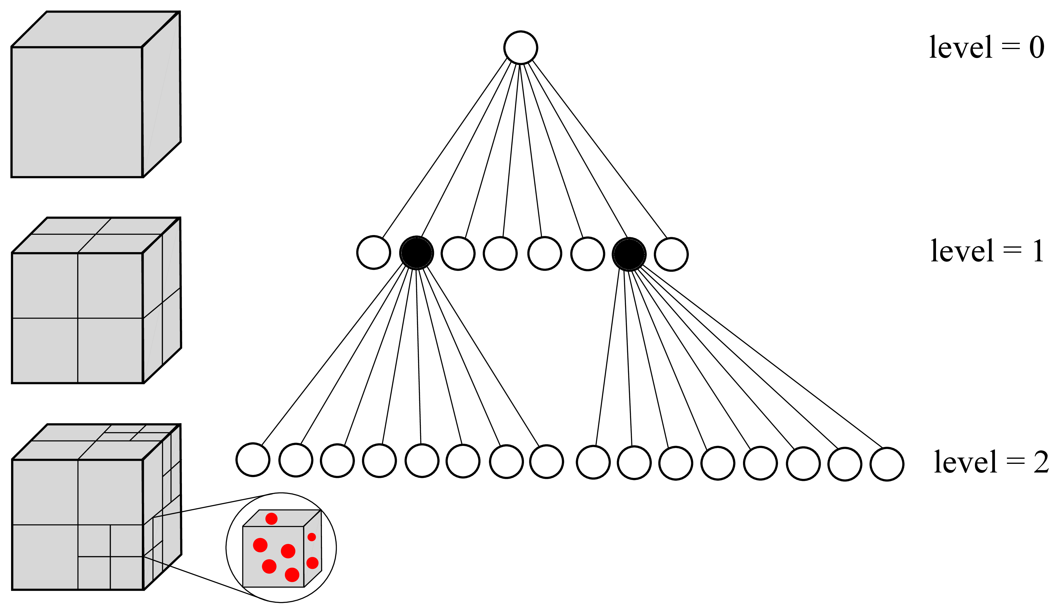
Figure: Simulation domain and its successive sub-branches on two levels, where particles are represented by red filled circles (left). Octree data structure depicting three levels of sub-divisions of the tree trunk (right).
Layer 2: Bounding sphere hierarchy
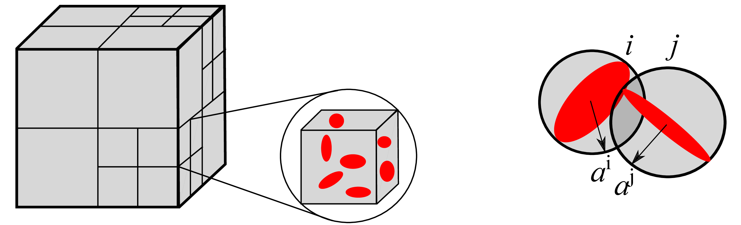
Figure: Upper layer consists of the Octree sub-branch with particles (left), and lower layer is defined by bounding spheres for particles \(i, j\) with radii \(a^i, a^j\) respectively (right).
Overlap detection
The actual overlap of two static ellipsoids is determined by the algebraic separation condition developed by Wang (2001). Consider two ellipsoids \(\mathcal{A}: \mathbf{X}^T \mathbf{A} \mathbf{X} = 0\) and \(\mathcal{B}: \mathbf{X}^T \mathbf{B} \mathbf{X} = 0\) in \(\mathbb{R}^3\), where \(\mathbf{X} = [x, y, z, 1]^T\), the characteristic equation is given as,
Wang et al. have established that the equation has at least two negative roots, and depending on the nature of the remaining two roots, the separation conditions are given as,
\(\mathbf{A}\) and \(\mathbf{B}\) are separated if \(f(\lambda) = 0\) has two distinct positive roots.
\(\mathbf{A}\) and \(\mathbf{B}\) touch externally if \(f(\lambda) = 0\) has a positive double root.
\(\mathbf{A}\) and \(\mathbf{B}\) overlap for all other cases.
Particle (Ellipsoid) packing
The user-defined simulation box size and the ellipsoid size distribution are used for creating the simulation box and ellipsoids. The simulation begins by randomly placing ellipsoids of null volume inside the box, and each ellipsoid is given a random velocity vector for movement. As the simulation proceeds, the ellipsoids grow in size along their axes and also collide with one another updating their position and velocities. The simulation terminates once all the ellipsoids have reached their defined volumes; the process is depicted pictorially in the figure below.
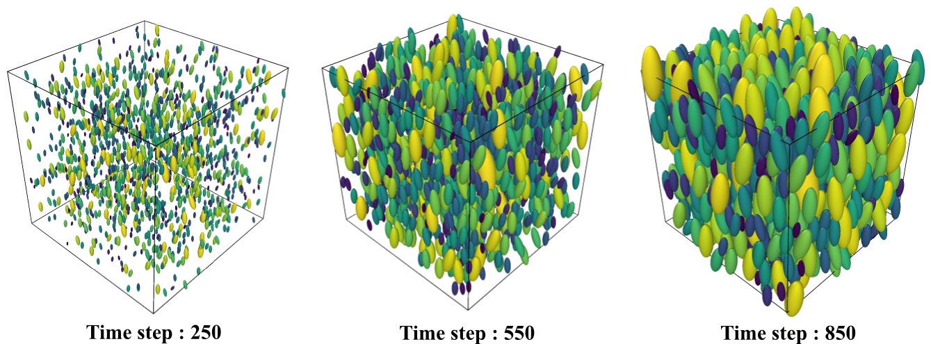
Figure: Ellipsoid packing simulation with partice interactions at three different timesteps.
Note
Since the application is microstructure generation, where all grains have a predefined tilt angle, the angular velocity vector \((\mathbf{w})\) is not considered for the ellipsoids and thus their orientations are constrained.
Texture
In this section a brief summary of the Orientation Distribution Function (ODF) reconstruction is presented. A detailed description of this can be found in Biswas (2020) as a \(L_1\) minimization scheme. Furthermore, an orientation assignment algorithm is presented which takes the grain boundary texture into consideration during the assignment process.
ODF reconstruction with discrete orientations
Crystallographic texture can be represented in the form of a continuous functions called ODF i.e., \(f:SO(3) \rightarrow \mathbb{R}\). With the availability of Electron Back Scatter Diffraction (EBSD) equipment, the polycrystalline materials are easily characterized in the form of measured crystallographic orientations \(g_i, \ i=1,...,N\).
The measured orientations \(g_i\) are used to estimate the ODF by a kernel density estimation Hielscher (2013). A bell shaped kernel function \(\psi: \ [0,\pi] \rightarrow \mathbb{R}\) is placed at each \(g_i\), which when combined together estimates the ODF as
where \(\omega(g_i , g)\) is the disorientation angle between the orientations \(g_i\) and \(g\). It is vital to note here that the estimated ODF \(f\) heavily depends on the choice of the kernel function \(\psi\). Keeping this in mind, the de la Vall'ee Poussin kernel \(\psi_\kappa\) is used for ODf reconstruction within Kanapy. Please refer to Schaeben (1997) for a detailed description of the de la Vall'ee Poussin kernel function as well as its advantages.
Within the numerical modeling framework for polycrystalline materials, the micromechanical modeling requires a reduced number \(N^\prime\) of discrete orientations \({g^\prime}_i\) to be assigned to grains in the RVE. The ODF of the reduced number of orientations is given as,
Since \(N^\prime \ll N\), the the kernel shape parameter \(\kappa\) must be optimized (\(\kappa^\prime\)) such that the ODF estimated from \({g^\prime}_i\) should be close to the input ODF \(f\). To quantify the difference between them an \(L_1\) error can be defined on the fixed \(SO(3)\) grid as
Orientation assignment process
In addition to the crystallographic texture, polycrystalline material also have grain boundary texture which is represented in the form of the misorientation distribution function (MDF). Similar to ODF, MDF can be estimated on \(\Delta \phi:SO(3) \rightarrow \mathbb{R}\) due to the disorientation (\(\Delta g_i, \ i=1,...,N_g\)) at grain boundary segments. These can be used to assign the discrete orientations obtained after ODF reconstruction to the grains in the RVE generated by Kanapy’s geometry module. Both the orientations and the disorientations play different roles in the mechanical behavior of the material, a detailed discussion of which can be found in Biswas (2019).
Other than the crystallographic orientation of the grains, the dimension of the grain boundary is also a key aspect. Therefore, to incorporate the effect of the grain boundary dimension, \(\Delta g\) at each segment is weighted as per the segment dimension, as suggested in Kocks (2000). Since the EBSD data is a 2D image this weighting factor is estimated as \(w_i = s_i/S\), where \(s_i\) is corresponding segment length and \(S = \sum_i^{N_g} s_i\).
The disorientation \(\Delta g\) can be represented in axis-angle notation. And within Kanapy’s algorithms we focus on the angle (\(\omega\)) part of \(\Delta g\), commonly referred to as the disorientation angle. To imitate the statistical distribution from experiments, a Monte-Carlo scheme is suggested in Miodownik (1999). This is used here in a \(L_1\) minimization framework similar to the ODF reconstruction discussed earlier.
The assignment algorithm begins by randomly assigning orientations obtained from ODF reconstruction to the grains in the RVE. The disorientation angle distribution is estimated in the present configuration including the weights (due to the corresponding grain boundaries) and the \(L_1\) error is estimated. The orientations are then exchanged between two grains modifying the configuration. The \(L_1\) error is estimated for the modified configuration, and compared with that of the previous configuration. If the error is minimized between the two configurations, then the orientations are retained, else the orientations are flipped to revert back to the previous configuration.
EBSD reading
Kanapy can read two dimensional EBSD maps and convert the measured pixel orientations into a graph representation of the microstructure. The graph is intended to describe the grain structure on the EBSD map after region segmentation, graph cleanup, and node merging. It can also be plotted directly on the EBSD inverse pole figure map for visual inspection.
The EBSD workflow is handled by kanapy.texture.EBSDmap. During map reading, Kanapy stores the EBSD pixel orientations, separates the retained phases, and builds graph data for the selected phase. For each phase, the graph data contains the final graph, diagnostic information from the initial graph, and merge information from the cleanup procedure.
Initial region construction
Initial EBSD regions are identified by local pixel to pixel misorientation. The procedure is implemented in kanapy.texture.find_similar_regions_by_misorientation(). Starting from each unassigned pixel, a breadth first search grows a region by adding neighboring pixels whose local misorientation is below the selected threshold. The misorientation calculation uses the crystal symmetry of the current phase.
For the two dimensional EBSD graph path, neighboring pixels are evaluated with 4-neighbor connectivity. This gives each pixel direct horizontal and vertical neighbors on the EBSD map. The resulting labeled regions form the initial graph nodes.
Graph construction and node data
The labeled EBSD regions are converted into graph nodes by kanapy.texture.build_graph_from_labeled_pixels(). Each graph node represents one connected labeled region. Node attributes include the pixel list, the node center, the number of pixels, the original pixel rotations, and the mean node orientation.
The mean orientation of a node is computed by kanapy.texture.mean_orientation_data(). Pixel quaternions are normalized, symmetry equivalent orientations are aligned to a reference orientation, and the q versus -q quaternion ambiguity is handled before averaging. The final mean quaternion is obtained from the dominant eigenvector of the quaternion accumulator matrix.
Graph edges are added between neighboring labeled regions. Label 0 is treated as background and is not used as a graph node.
Boundary artifact cleanup
Some small regions can appear mainly along grain boundaries. Kanapy computes node boundary information with kanapy.texture.get_node_boundary_stats(). For each node, the function checks local neighboring pixels and reports boundary pixel fraction, neighboring labels, map edge contact, bounding box size, and bounding box fill fraction.
Small boundary artifact nodes can be merged with kanapy.texture.merge_boundary_artifact_nodes(). The merge target is chosen from neighboring nodes by comparing the node orientations. After node merging, the mean orientation of the merged node is recomputed from the original pixel orientations.
Graph plotting
The final EBSD graph can be plotted on the EBSD inverse pole figure map by setting show_graph=True when creating an kanapy.texture.EBSDmap object. The graph overlay is produced by kanapy.texture.EBSDmap.plot_graph_overlay(). Node centers are shown as black points and graph edges are shown as black lines.
Example usage:
import kanapy as knpy

ebsd = knpy.EBSDmap("p558_250x_1.ang", show_graph=True)
The same plotting method can also save the graph image to file when an output path is provided.
Example script
The graph workflow example is provided in examples/EBSD_graph_analysis.
run_ebsd_analysis_with_graph.pyBuilds an in memory
kanapy.graph_workflow.EBSDGraphResultobject and writes only the explicitly enabled graph handoff files. This example uses the graph only path and does not run grain statistics extraction or the legacy interactive plotting workflow. The output is written to2D_graph_result.
The graph workflow can be called directly from Python by using kanapy.graph_workflow.build_ebsd_graph(). The main data transfer object is kanapy.graph_workflow.EBSDGraphResult; PKL, JSON, and PNG files are written only when enabled through kanapy.graph_workflow.EBSDGraphOutputOptions. Users who need the classic EBSD statistics and interactive Kanapy plots can still create kanapy.texture.EBSDmap directly with the usual plotting flags.
The example keeps graph step figures and local zoom diagnostics disabled by default. These outputs are mainly useful for debugging or preparing publication figures, while routine workflows usually need only the final graph handoff files.
The graph workflow example produces:
2D_graph_result/ebsd_graph.pkl
2D_graph_result/ebsd_graph_summary.json
2D_graph_result/graph_overlay.png
2D_graph_result/graph_ipf_map.png
The overlay image shows the final graph node centers and graph edges on the EBSD inverse pole figure map.